Getting familiar with the R2D2 prior for GLMMs
Introduction
This blog post exists because I really wanted to write another blog post, not this one. But life is full of surprises, I have to say.
I just wanted to replicate some results in Yanchenko et al. (2024), the paper that introduces the R2D2 prior for Generalized Linear Mixed Models (GLMMs). I would read the math, implement what I needed, use PyMC to build a model, obtain a posterior, and write down a couple of conclusions. That would be it.
While working through the paper, I got completely drawn into it: I found myself re-reading sections several times and implementing almost everything in code. Now, I do feel I can explain how it works in a few minutes, but it took me many hours to grasp the core ideas. Along the way, I wrote a lot of code, examples, and tests that, unfortunately, don’t really fit into the original blog post.
So here we are, ending up with this extra post. It is one that doesn’t include much code. Instead, it focuses on the explanation I was able to distill while experimenting with this prior. If you prefer to learn by looking at (and playing with) code, feel free to look at this gist, which contains all the code behind the post.
Otherwise, welcome! This is my attempt to explain R2D2 for GLMMs, share a few experiments I ran, and wrap up with some conclusions.
R2D2 for normal regression
The R2D2 prior for normal regression models has been introduced in Zhang et al. (2020).
Consider the normal regression model:
\[ \begin{aligned} Y_i \mid \mu_i, \sigma^2 &\underset{iid}{\sim} \text{Normal}(\mu_i, \sigma^2) \\ \mu_i &= \alpha + \beta_1 X_{1i} + \beta_2 X_{2i} + \dots + \beta_p X_{pi} \\ &= \alpha + \boldsymbol{X}\boldsymbol{\beta} \end{aligned} \]
where \(\boldsymbol{X}\) is the design matrix, \(\alpha\) is the intercept term, and \(\boldsymbol{\beta}\) is the vector of coefficients.
The central idea in the R2D2 prior is to place a prior directly on the coefficient of determination \(R^2\). For the purpose of defining prior distributions, the authors work with the marginal coefficient of determination: a version of \(R^2\) that averages over both the design matrix \(\boldsymbol{X}\) and the regression coefficients \(\boldsymbol{\beta}\).
For the linear regression model, the marginal \(R^2\) is defined as:
\[ R^2 = \frac{\mathbb{V}(\boldsymbol{x}^T \boldsymbol{\beta})}{\mathbb{V}(\boldsymbol{x}^T \boldsymbol{\beta}) + \sigma^2} = \frac{\sigma^2 W}{\sigma^2 W + \sigma^2} = \frac{W}{W + 1} \]
which is the ratio of the marginal variance of the linear predictor to the marginal variance of the outcome.
Then, the R2D2 prior is specified as:
\[ \begin{aligned} \beta_j \mid \phi_j, W, \sigma^2 &\sim \text{Normal}(0, \phi_j W \sigma^2) \\ \boldsymbol{\phi} &\sim \text{Dirichlet}(\xi_1, \dots, \xi_p) \\ W & = \frac{R^2}{1 - R^2}\\ R^2 &\sim \text{Beta}(a, b) \\ \end{aligned} \]
The prior on \(R^2\) induces a prior on \(W\), which governs the total prior variance of the linear predictor \(\boldsymbol{x}^T \boldsymbol{\beta}\). Combined with the Dirichlet prior on the variance proportions \(\boldsymbol{\phi}\), this results in the \(R^2\)-induced Dirichlet Decomposition (R2D2) prior.
It can be shown that the induced prior on \(W\) is a Beta Prime distribution with parameters \(a\) and \(b\).
R2D2 for GLMMs
Suppose we have a GLMM of the form:
\[ \begin{aligned} Y_i \mid \mu_i, \theta &\underset{iid}{\sim} \mathcal{F}(\mu_i, \theta) \\ g(\mu_i) &= \eta_i = \alpha + \boldsymbol{x}_i \boldsymbol{\beta} + \sum_{k=1}^{q}u_{k g_k[i]} \\ \end{aligned} \]
There are \(n\) observations indexed by \(i \in \{1,\dots,n\}\). The response variable for observation \(i\) is denoted \(Y_i\), with mean \(\mu_i\). Conditional on \(\mu_i\), and possibly additional parameters \(\theta\), the response variables \(Y_i\) are assumed to be independent and identically distributed (\(\mathcal{F}\) represents an arbitrary family). A link function \(g(\cdot)\) relates the mean \(\mu_i\) to the linear predictor \(\eta_i\).
The linear predictor consists of an intercept \(\alpha\), \(p\) explanatory variables, and \(q\) types of random effects. For the \(i\)-th observation, the covariates are collected in the vector \(\boldsymbol{x}_i = (x_{i1},\dots,x_{ip})\), and the full set of covariates for all observations forms the design matrix \(\boldsymbol{X}\), of dimension \(n \times p\). It is assumed that \(\boldsymbol{X}\) has been standardized so that each column has mean zero and variance one.
The fixed-effect coefficients form the vector \(\boldsymbol{\beta} = (\beta_1, \dots, \beta_p)^T\). For the \(k\)-th random effect, there are \(L_k\) levels collected in \(\boldsymbol{u}_k = (u_{k1},\dots,u_{kL_k})^T\), and we use \(g_k[i]\) indicate the level of the random effect \(k\) for the observation \(i\).
To construct the R2D2 prior for GLMMs, Yanchenko et al. (2024) specify the following prior model:
\[ \begin{aligned} \beta_j \mid \phi_j, W &\sim\text{Normal}(0, \phi_j W) \\ \boldsymbol{u}_k \mid \phi_{p + k}, W &\sim\text{Normal}(0, \phi_{p + k}W \boldsymbol{I}_{L_k}) \end{aligned} \]
The parameter \(W > 0\) governs the overall variance of the linear predictor, controlling the total amount of variation in the fixed and random effects. Larger values of \(W\) correspond to more flexible models, while smaller values shrink the model toward an intercept-only model.
The parameters \(\phi_j \ge 0\), which satisfy \(\sum_{j=1}^{p+q} \phi_j = 1\), determine how this total variance \(W\) is distributed across the individual fixed and random effect components. The vector of variance proportions \(\boldsymbol{\phi} = (\phi_1,\dots,\phi_{p+q})\) is typically given a Dirichlet prior,
\[ \boldsymbol{\phi} \sim \text{Dirichlet}(\xi_1, \dots, \xi_{p+q}), \]
and in many applications all concentration parameters are set to a common value \(\xi_0\). Larger values of \(\xi_0\) shrink the variance proportions toward the uniform allocation \(1 / (p+q)\), while smaller values allow for more dispersed and uncertain allocations across components.
Like in the linear model case, the R2D2 prior for GLMMs is specified by placing a prior on the marginal \(R^2\) that averages over explanatory variables and random effects (\(\boldsymbol{X}\) and \(\boldsymbol{g}\)) as well as parameters (\(\boldsymbol{\beta}\) and \(\boldsymbol{u}_k\)).
This marginal \(R^2\) is defined as:
\[ R^2 = \frac{\mathbb{V}(\mathbb{E}(Y \mid \eta))}{\mathbb{V}(\mathbb{E}(Y \mid \eta)) + \mathbb{E}(\mathbb{V}(Y \mid \eta))} \]
Given that \(R^2\) is based on summaries of the distribution of the linear predictor \(\eta\), and it is assumed that \(\eta_i \mid \alpha, W \sim \text{Normal}(\alpha, W)\), \(R^2\) also depends on the parameters \(\alpha\) and \(W\).
The details
The essence of the R2D2 prior for GLMMs is to define a joint prior on \((\alpha, W)\) such that the resulting induced prior on \(R^2\) is \(\text{Beta}(a, b)\).
Yanchenko et al. (2024) construct such a prior by decomposing the joint distribution into a marginal prior for \(\alpha\) and a conditional prior for \(W \mid \alpha\). They then choose a prior for \(W \mid \alpha\) that ensures the induced distribution of \(R^2\) is \(\text{Beta}(a, b)\) for any fixed value of \(\alpha\). Because this holds conditionally for all \(\alpha\), the marginal distribution of \(R^2\) under the joint prior on \((\alpha, W)\) is also \(\text{Beta}(a, b)\), regardless of the marginal prior placed on \(\alpha\). Combined with a Dirichlet prior on the variance proportions, this construction yields the R2D2 prior for GLMMs.
The need for approximations
For some model families, the prior on \(W\) that induces \(R^2 \sim \text{Beta}(a, b)\) can be derived in closed form. However, since this is not generally possible for GLMMs, the authors propose a unified approximate approach that works across all model families.
The idea is to place a Generalized Beta Prime (GBP) prior on \(W\) and choose its parameters so that the resulting induced distribution of \(R^2\) closely matches the target \(\text{Beta}(a, b)\) distribution.
The problem becomes finding the values \((a^*, b^*, c^*, d^*)\) so that the prior \(W \sim \text{GBP}(a^*, b^*, c^*, d^*)\) induces a prior on \(R^2\) that is close to \(\text{Beta}(a, b)\).
Suppose \(p(w)\) is the density function of the distribution on \(W\) that yields exactly \(R^2 \sim \text{Beta}(a, b)\). To obtain the values of the parameters of the GBP distribution, the authors minimize the Pearson \(\chi^2\) divergence between the true density \(p(w)\) and its GBP approximation \(p_{GBP}(w)\), with an added regularization term that shrinks the solution toward \(\text{GBP}(a^*, b^*, 1, 1)\), which is the exact solution for certain model families and can be considered the baseline.
The optimization problem is formulated as:
\[ \begin{aligned} (a^*, b^*, c^*, d^*) & = \arg\min_{\alpha, \beta, c, d} \int_0^{\infty} \left\{ \frac{p_{GBP}(w, \alpha, \beta, c, d) - p(w)}{p(w)} \right\}^2 p(w) dw \\ & \qquad \qquad \quad + \quad \lambda \left[(\alpha - a)^2 + (\beta - b)^2 + (c - 1)^2 + (d - 1)^2\right] \end{aligned} \]
Here, \(\lambda \ge 0\) is a tuning parameter that controls the amount of the regularization, which the authors suggest setting to \(\lambda = 1 / 4\).
How to use it
In practice, specifying the R2D2 prior for GLMMs requires the user to choose the Beta hyperparameters \(a\) and \(b\) for the desired prior on \(R^2\). One then solves the optimization problem above to find the parameters \((a^*, b^*, c^*, d^*)\) of the GBP prior on \(W\).
The resulting prior can be implemented via the transformation:
\[ V \sim \text{Beta}(a^*, b^*) \implies W = d^*\left[\frac{V}{1 - V}\right]^{1/c^*} \sim \text{GBP}(a^*, b^*, c^*, d^*) \]
When doing inference with MCMC, because the optimal values \((a^*, b^*, c^*, d^*)\) depend on \(\alpha\) and possibly other response-distribution parameters \(\theta\), the approximation should be updated with their values at every iteration.
However, performing the optimization at every MCMC iteration would be computationally infeasible. To address this, the authors recommend computing the GBP approximation once at the start of the analysis using \(\hat{\alpha} = g(\bar{Y}_i)\) and, if needed, the maximum likelihood estimate \(\hat{\theta}\). Once the values of \((a^*, b^*, c^*, d^*)\) are found, \(\alpha\) and \(\theta\) are treated as unknown again during the subsequent Bayesian inference.
Python implementation
Below I include a bare-bones implementation of a function that computes \((a^*, b^*, c^*, d^*)\) for the GBP approximation corresponding to a desired \(\text{Beta}(a, b)\) prior on \(R^2\). Its purpose is simply to show that minimizing the divergence is not the tedious part; dealing with all the details across different model families is.
If you want to see the actual code, including all the rough edges and unpleasant implementation details, have a look at this gist.
Code: Basic implementation
import numpy as np
from scipy import special
from scipy.optimize import minimize

def penalized_divergence(p_true, p_approx, params_current, params_reference, lam):
    """Penalized Pearson Chi-squared divergence"""
    integral = np.sum((1 - p_approx / p_true) ** 2)
    penalty = lam * np.sum((params_current - params_reference) ** 2)
    return integral + penalty


def gbp_pdf(x, a, b, c, d):
    """Probability density function of the GBP distribution"""
    log_num = (
        np.log(c)
        + (a * c - 1) * (np.log(x) - np.log(d))
        - (a + b) * np.log1p((x / d) ** c)
    )
    log_den = np.log(d) + special.betaln(a, b)
    return np.exp(log_num - log_den)


def WGBP(a, b, w_grid, p_true, lam=0.25, initial_point=np.ones(4)):
    """Compute parameters for the GBP Approximation

    Estimate the parameters of the Generalized Beta Prime (GBP) approximation to the
    distribution of W induced by a Beta(a, b) prior on R².
    Parameters
    ----------
    a : float
        First parameter of the Beta(a, b) prior on R².
    b : float
        Second parameter of the Beta(a, b) prior on R².
    w_grid : np.ndarray
        One-dimensional grid of W values where the true and approximate densities are
        evaluated.
    p_true : callable
        Function that returns the true density p(w) when called on `w_grid`.
    lam : float, optional
        Penalization weight for regularization (default 0.25).
    initial_point : np.ndarray, optional
        Initial guess for the optimization procedure (default: np.ones(4)).

    Returns
    -------
    np.ndarray
        Array with the estimated GBP parameters (a*, b*, c*, d*)
        that approximate the true density of W.
    """

    params_reference = np.array([a, b, 1, 1])
    def divergence(params):
        return penalized_divergence(
            p_true=p_true(w_grid),
            p_approx=gbp_pdf(w_grid, *params),
            params_current=params,
            params_reference=params_reference,
            lam=lam
        )

    result = minimize(divergence, x0=initial_point)

    if result.success:
        return result.x

    raise Exception("Minimization didn't converge")
Experimental results
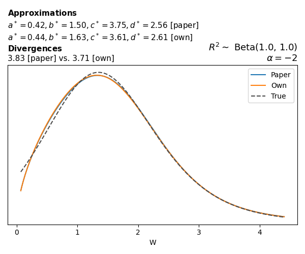
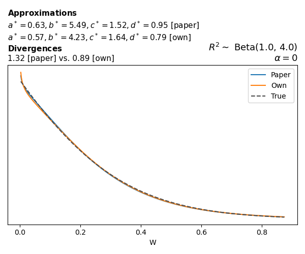
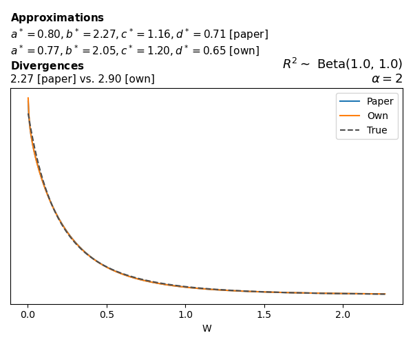
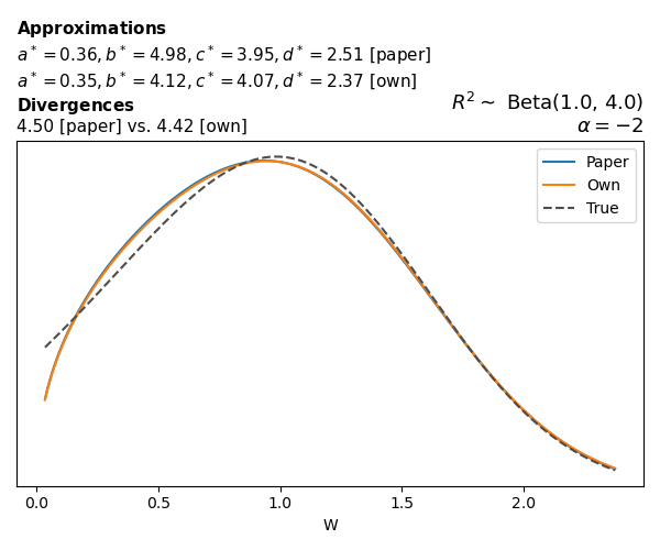
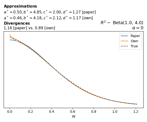
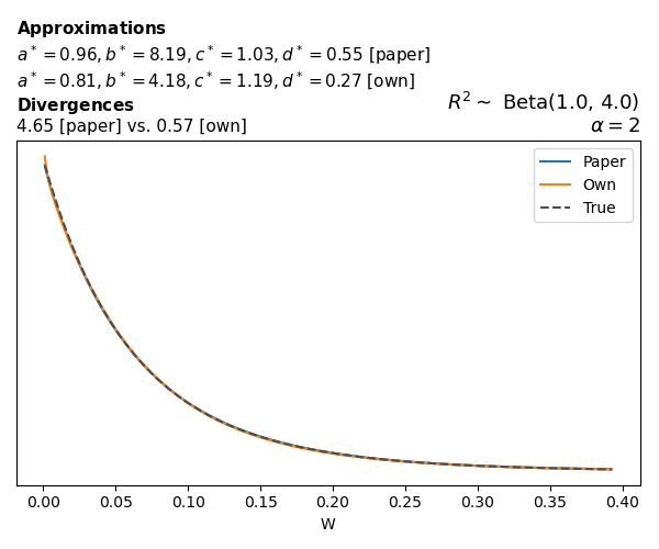
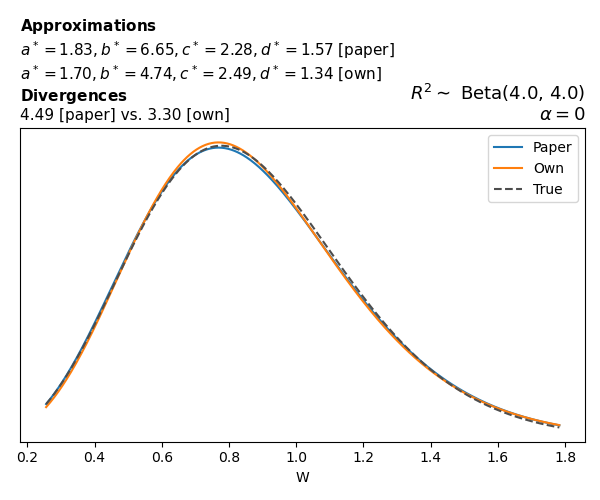
To evaluate my implementation of the function that computes the hyperparameters of the Generalized Beta Prime distribution, I reproduced the results from Table 5 in Yanchenko et al. (2024) (shown below).
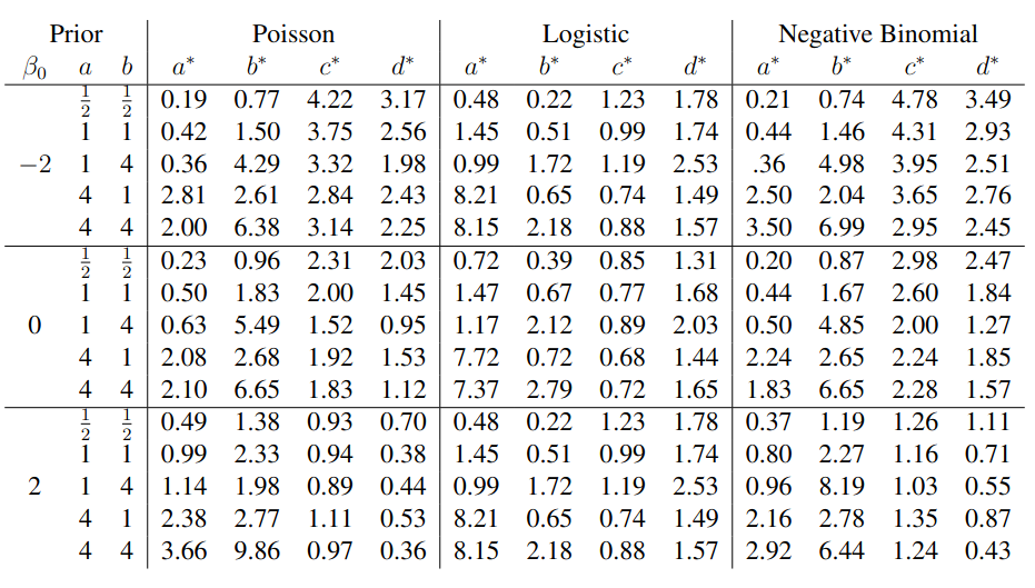
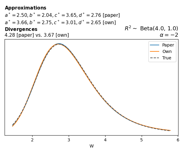
In what follows, we will examine, for three model families and for all combinations of \(a\), \(b\), and the intercept (denoted \(\alpha\) in my code and \(\beta_0\) in the paper), the following:
In what follows, we will see, for three model families, and for all settings of \(a\), \(b\), and intercept (\(\alpha\) in my case, \(\beta_0\) in the paper):
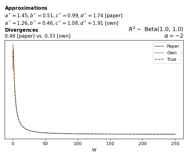
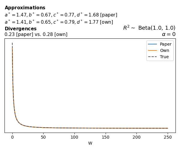
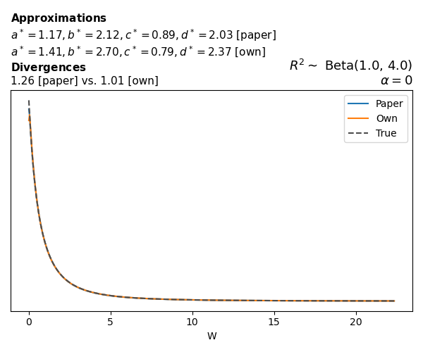
- the true probability density function of \(W\)
- the GBP approximation reported in the paper
- the GBP approximation obtained from my implementation
- the divergence between each approximation and the true density
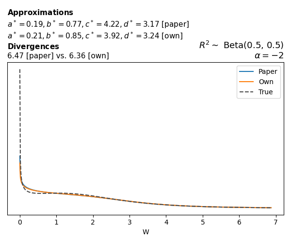
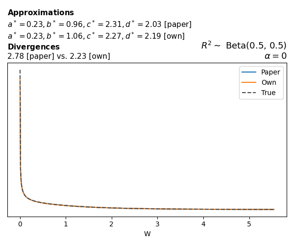
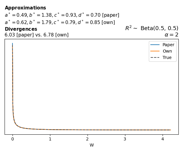
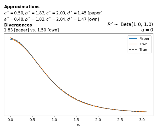
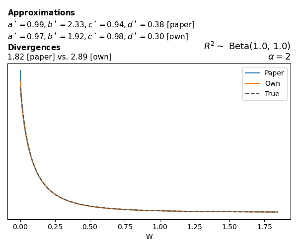
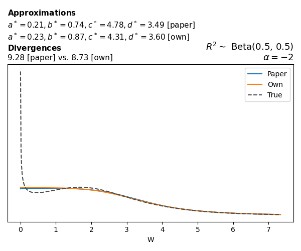
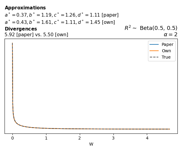
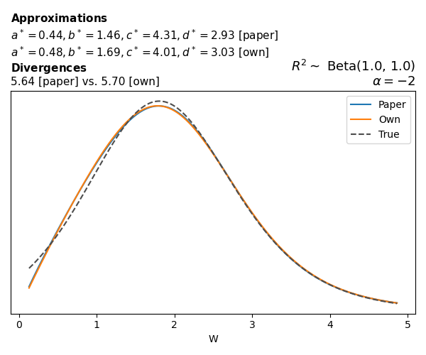
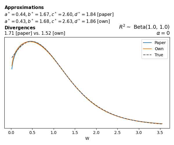
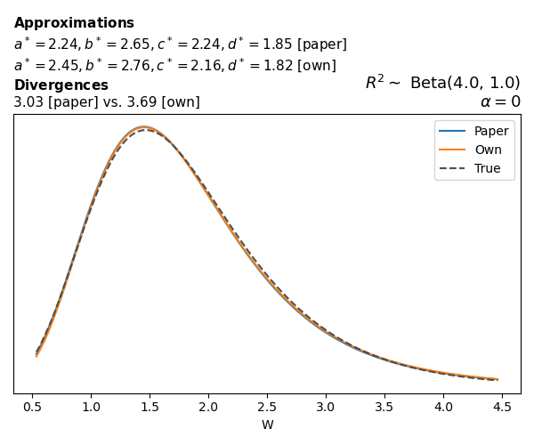
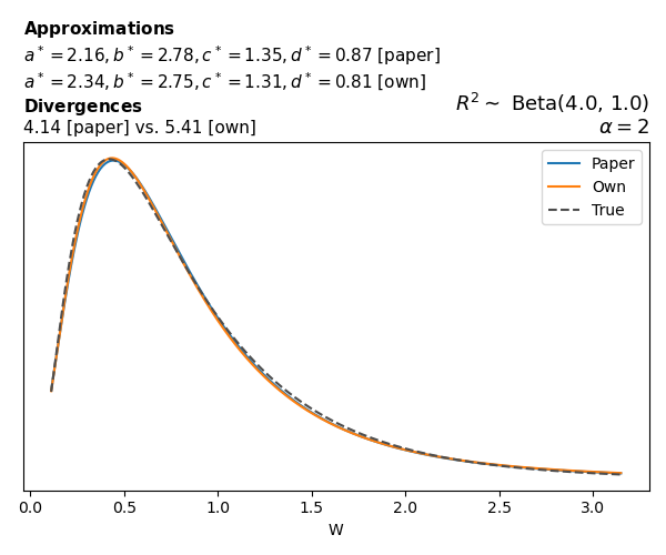
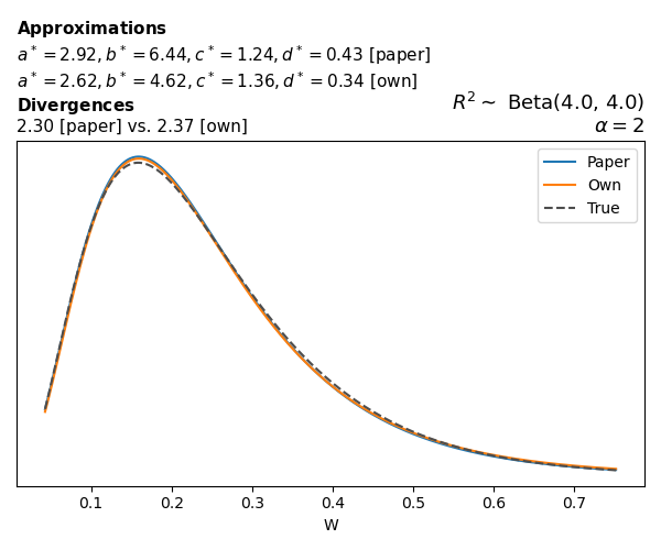
Poisson
The relationship between \(W\) and \(R^2\), as well as the probability density function of \(W\), in the case of a Poisson regression model with a log link function, are given in Equations 7 and 8 of Yanchenko et al. (2024).
\[ \begin{aligned} R^2 &= \frac{e^W - 1}{e^W - 1 + e^{-\alpha - \frac{1}{2} W}} \\ \\ p(w \mid \alpha, a, b) &= \frac{1}{2B(a, b)} \frac {(e^w - 1)^{a - 1} e^{-b(\alpha+ w/2)} (3e^w-1)} {(e^w - 1 + e^{-\alpha - w/2})^{a+b}}, \qquad w \ge 0. \end{aligned} \]
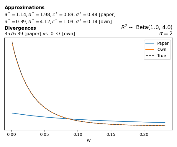
I suspect there's a transcription error
in the paper for this
example
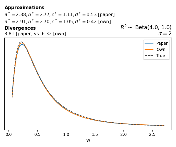
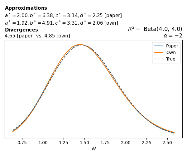
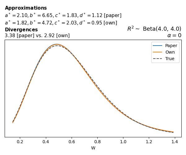
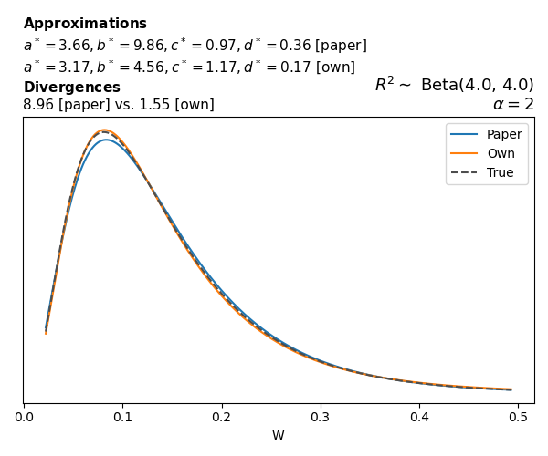
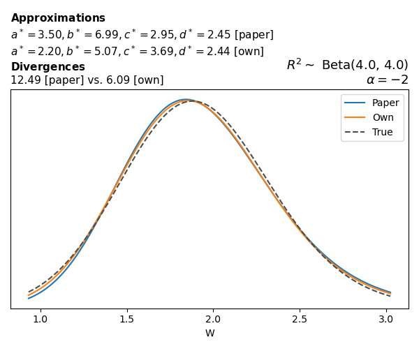
We can highlight a few things:
- The specific hyperparameters I obtain are never exactly the same as the ones in the paper.
- However, the resulting GBP distributions are, in general, qualitatively similar.
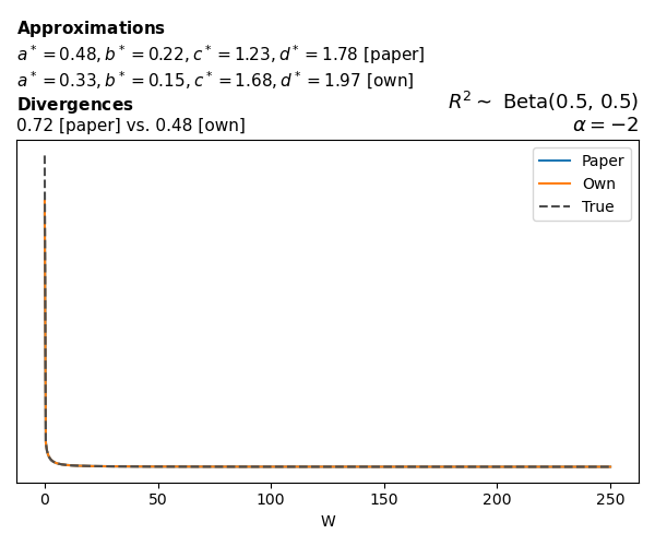
- \(\text{Beta}\) priors with \(a=0.5\) and \(b=0.5\) yield priors on \(W\) with a sharp peak near zero and very heavy tails.
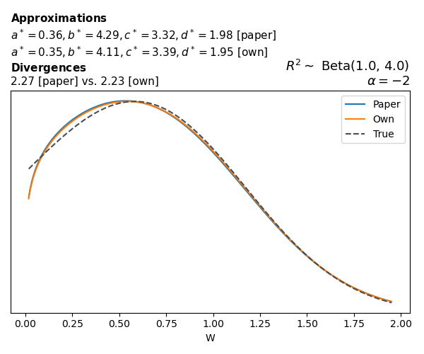
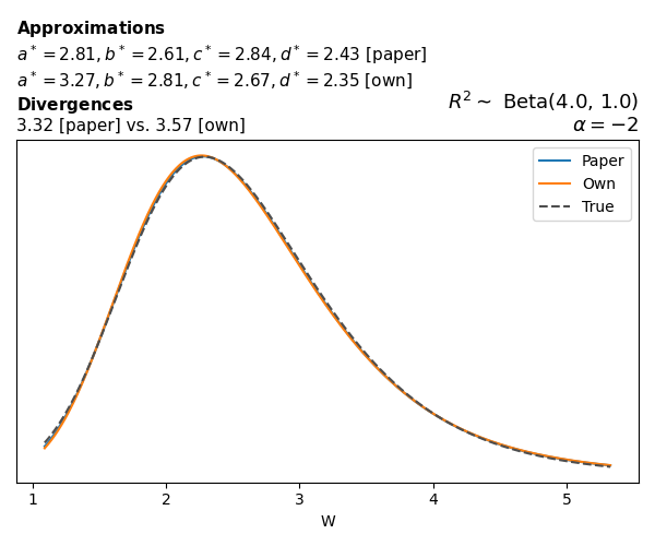
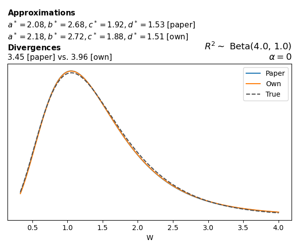
Negative binomial
In the case of negative binomial regression, again with a log link function, we also have to consider the overdispersion parameter \(\theta > 1\). Equations 23 and 24 in Yanchenko et al. (2024) show:
\[ \begin{aligned} R^2 &= \frac{e^W - 1}{e^W - 1 + \theta e^{-\alpha - \frac{1}{2} W}} \\ \\ p(w \mid \alpha, a, b) &= \frac{\theta^b}{2B(a, b)} \frac {(e^w - 1)^{a - 1} e^{-b(\alpha+ w/2)} (3e^w-1)} {(e^w - 1 + \theta e^{-\alpha - w/2})^{a+b}}, \qquad w \ge 0. \end{aligned} \]

The conclusions are similar to the ones I wrote above.
Logistic
Closed-form expressions are not available for logistic regression with a logit link. If you’re insterested in the details, have a look at the callouts below.
Yanchenko et al. (2024) approximates the coefficient of determination \(R^2\) for given \(W\) and \(\alpha\) using a quasi–Monte Carlo method. Their approximation, denoted \(\tilde{R}^2\), is given by
\[ \tilde{R}^2(W \mid \alpha) \approx \frac{ \tilde{\mu}_2(W \mid \alpha) - \tilde{\mu}_1^2(W \mid \alpha) } { \tilde{\mu}_2(W \mid \alpha) - \tilde{\mu}_1^2(W \mid \alpha) + \tilde{\sigma}^2(W \mid \alpha) } \]
To compute this approximation, we need estimates of the conditional moments of the latent variable \(\eta = \alpha + z \sqrt{W}\):
\[ \mathrm{E}\{\mu(\eta)^m\} \approx \tilde{\mu}_m(W \mid \alpha) = \frac{1}{K-1} \sum_{i=1}^{K-1} \mu(\alpha + z_i \sqrt{W})^m, \]
and
\[ \mathrm{E}\{\sigma^2(\eta)\} \approx \tilde{\sigma}^2(W \mid \alpha) = \frac{1}{K-1} \sum_{i=1}^{K-1} \sigma^2(\alpha + z_i \sqrt{W}) \]
where \(z_i\) is the \(i/K\) quantile of a standard normal distribution, with \(K\) being the number of quantiles used in the approximation. The functions \(\mu\) and \(\sigma^2\) represent:
\[ \begin{aligned} \mu(\eta) &= \mathbb{E}(Y \mid \eta) \\ \sigma^2(\eta) &= \mathbb{V}(Y \mid \eta) \end{aligned} \]
which are
\[ \begin{aligned} \mu(\eta) &= \text{expit}(\eta) \\ \sigma^2(\eta) &= \mu(\eta) \cdot (1 - \mu(\eta)) \end{aligned} \]
in the case of the logistic regression family.
The PDF is the derivative of the CDF, \[ p(w) = \frac{d}{dw} F(w). \]
Since no closed form is available, we approximate the derivative using a central finite difference, for a small \(\delta>0\):
\[ p(w) \approx \frac{F(w + \delta) - F(w - \delta)}{2 \delta} \]
Here the CDF of \(W\) is computed by first approximating the corresponding \(R^2\) value from \(W\), and then evaluating the Beta CDF of \(R^2\).
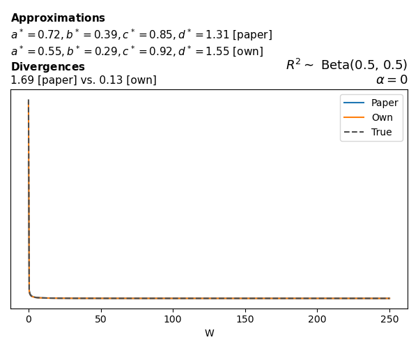


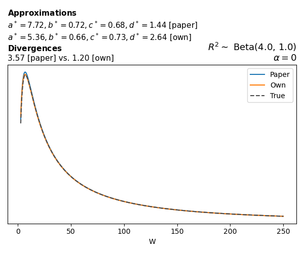


The main, and rather obvious, conclusion is that all resulting priors on \(W\) are very heavy-tailed. When you see the horizontal axis extending all the way to 250, that’s only because I manually reduced its upper bound.
Other than that, the approximation seems to work reasonably well, although I’m not entirely sure how good my judgement is here (after all, my approximation is approximating another approximation!).
Final thoughts
Well, it seems I’m done, at least for now. I’m really glad I managed to build a Python implementation that lets me use the R2D2 prior in GLMMs. Before wrapping up, let me share a few concluding notes.
While experimenting with different values of \(a\) and \(b\), I noticed that \(\text{Beta}(0.5,0.5)\) induces a prior on \(W\) with most of its mass near zero and heavy tails. I don’t think this is a great choice, other than for testing purposes. Even the uniform \(\text{Beta}(1,1)\) is not obviously preferable. Alternatives that are moderately informative such as \(\text{Beta}(2,2)\) or \(\text{Beta}(4,4)\) already induce a smoother prior on \(W\).
Regarding specific families, I noticed that for the Poisson and negative binomial models the prior mass tends to concentrate near the origin as the intercept varies (from \(-2\) to \(0\) and from \(0\) to \(2\)), although I still do not fully understand why. In the logistic case, the (approximate) prior on \(W\) has extremely heavy tails, which I don’t think is desirable.
From an implementation perspective, there were also a few surprises. The actual value of the divergence turns out to be very sensitive to the choice of the grid over \(w\), and it is easy to tweak a setting and obtain different values for \((a^*, b^*, c^*, d^*)\). Avoiding numerical issues was also not trivial, especially for heavy-tailed families such as the logistic one. If you read the code, you will probably notice several small “robustification” tricks that were necessary to make everything work.
What’s next
And now? Time to write the blog post I originally intended to write: using the R2D2 prior in GLMMs with PyMC. Hopefully I’ll be able to finish that one soon!