Code
import arviz as az
import matplotlib.pyplot as plt
import numpy as np
import polars as pl
import pymc as pm
import pytensor.tensor as pt

c_orange = "#f08533"
c_blue = "#3b78b0"
c_red = "#d1352c"NOTE: You also have this versión en español.
import arviz as az
import matplotlib.pyplot as plt
import numpy as np
import polars as pl
import pymc as pm
import pytensor.tensor as pt
c_orange = "#f08533"
c_blue = "#3b78b0"
c_red = "#d1352c"While I was scraping data on NBA rookies’ free throws during the 2024–25 season, I came across this article, which concludes that there’s a “warm-up” effect: basketball players tend to miss their first shots more often than the rest. I found the result both interesting and intuitive, and it made me wonder whether it would be worth running a similar analysis on the data I was collecting.
And well… here we are.
The following data frame contains information about the free throws taken by NBA rookies during the 2024–25 season. In this case, the relevant columns are the player’s identifier (player_id), the order of the attempt (description), and whether the shot was made (success).
df = (
    pl.read_parquet("data.parquet")
    .select("game_date", "matchup", "player_id", "player_name", "description", "success")
)
df| game_date | matchup | player_id | player_name | description | success |
|---|---|---|---|---|---|
| date | str | i32 | str | str | bool |
| 2025-04-05 | "MEM @ DET" | 1641744 | "Edey, Zach" | "Free Throw 1 of 2" | false |
| 2025-04-05 | "MEM @ DET" | 1641744 | "Edey, Zach" | "Free Throw 2 of 2" | false |
| 2025-01-18 | "PHI @ IND" | 1641737 | "Bona, Adem" | "Free Throw 1 of 1" | true |
| 2025-01-18 | "PHI @ IND" | 1641737 | "Bona, Adem" | "Free Throw 1 of 2" | false |
| 2025-01-18 | "PHI @ IND" | 1641737 | "Bona, Adem" | "Free Throw 2 of 2" | true |
| … | … | … | … | … | … |
| 2024-11-06 | "MEM vs. LAL" | 1642530 | "Kawamura, Yuki" | "Free Throw 1 of 2" | true |
| 2024-11-06 | "MEM vs. LAL" | 1642530 | "Kawamura, Yuki" | "Free Throw 2 of 2" | true |
| 2025-03-12 | "MEM vs. UTA" | 1641744 | "Edey, Zach" | "Free Throw 1 of 1" | false |
| 2024-11-22 | "NOP vs. GSW" | 1641810 | "Reeves, Antonio" | "Free Throw 1 of 2" | true |
| 2024-11-22 | "NOP vs. GSW" | 1641810 | "Reeves, Antonio" | "Free Throw 2 of 2" | false |
In the NBA, free throws can come in series of 1, 2, or 3 attempts. Our first task is to map the values of description to a numeric value representing the order of the shot within its series.
throw_order = {
    "Free Throw 1 of 1": 1,
    "Free Throw 1 of 2": 1,
    "Free Throw 1 of 3": 1,
    "Free Throw 2 of 2": 2,
    "Free Throw 2 of 3": 2,
    "Free Throw 3 of 3": 3,
    "Free Throw Clear Path 1 of 2": 1,
    "Free Throw Clear Path 2 of 2": 2,
    "Free Throw Flagrant 1 of 1": 1,
    "Free Throw Flagrant 1 of 2": 1,
    "Free Throw Flagrant 2 of 2": 2,
    "Free Throw Technical": 1,
}

df = df.with_columns(
    pl.col("description").replace_strict(throw_order, return_dtype=pl.Int64).alias("order")
)
df| game_date | matchup | player_id | player_name | description | success | order |
|---|---|---|---|---|---|---|
| date | str | i32 | str | str | bool | i64 |
| 2025-04-05 | "MEM @ DET" | 1641744 | "Edey, Zach" | "Free Throw 1 of 2" | false | 1 |
| 2025-04-05 | "MEM @ DET" | 1641744 | "Edey, Zach" | "Free Throw 2 of 2" | false | 2 |
| 2025-01-18 | "PHI @ IND" | 1641737 | "Bona, Adem" | "Free Throw 1 of 1" | true | 1 |
| 2025-01-18 | "PHI @ IND" | 1641737 | "Bona, Adem" | "Free Throw 1 of 2" | false | 1 |
| 2025-01-18 | "PHI @ IND" | 1641737 | "Bona, Adem" | "Free Throw 2 of 2" | true | 2 |
| … | … | … | … | … | … | … |
| 2024-11-06 | "MEM vs. LAL" | 1642530 | "Kawamura, Yuki" | "Free Throw 1 of 2" | true | 1 |
| 2024-11-06 | "MEM vs. LAL" | 1642530 | "Kawamura, Yuki" | "Free Throw 2 of 2" | true | 2 |
| 2025-03-12 | "MEM vs. UTA" | 1641744 | "Edey, Zach" | "Free Throw 1 of 1" | false | 1 |
| 2024-11-22 | "NOP vs. GSW" | 1641810 | "Reeves, Antonio" | "Free Throw 1 of 2" | true | 1 |
| 2024-11-22 | "NOP vs. GSW" | 1641810 | "Reeves, Antonio" | "Free Throw 2 of 2" | false | 2 |
We can see that first attempts tend to miss more often than second ones — and second attempts, in turn, miss more often than third ones.
df_summary = (
    df
    .group_by("order")
    .agg(pl.col("success").sum().alias("y"), pl.len().alias("n"))
    .with_columns((pl.col("y") / pl.col("n")).alias("p"))
    .sort("order")
)
df_summary| order | y | n | p |
|---|---|---|---|
| i64 | u32 | u32 | f64 |
| 1 | 1435 | 2069 | 0.693572 |
| 2 | 1227 | 1625 | 0.755077 |
| 3 | 23 | 28 | 0.821429 |
As a first step, we use a model that groups all players’ shots together and treats them as equivalent — more of the same. We define \(Y_1\) as the number of made first attempts and \(Y_2\) as the number of made second attempts. Then, \(\pi_1\) represents the probability of making a first attempt, and \(\pi_2\) the probability of making a second one.
\[ \begin{aligned} Y_1 &\sim \text{Binomial}(N_1, \pi_1) \\ Y_2 &\sim \text{Binomial}(N_2, \pi_2) \\ \pi_1 &\sim \text{Beta}(4, 2) \\ \pi_2 &\sim \text{Beta}(4, 2) \\ \end{aligned} \]
In PyMC, we have:
y = df_summary.head(2)["y"].to_numpy()
n = df_summary.head(2)["n"].to_numpy()

with pm.Model(coords={"order": [1, 2]}) as model:
    pi = pm.Beta("pi", alpha=4, beta=2, dims="order")
    y = pm.Binomial("y", p=pi, n=n, observed=y, dims="order")
    idata = pm.sample(chains=4, random_seed=1211, nuts_sampler="nutpie", progressbar=False)

model.to_graphviz()
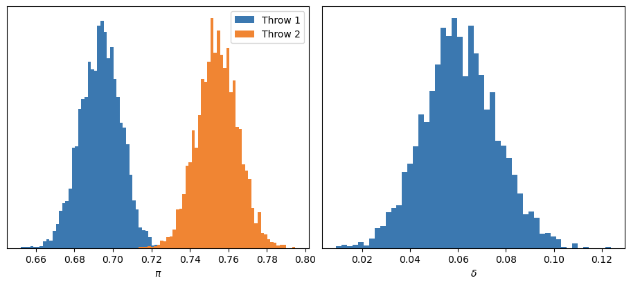
We compute \(\delta\) as the difference between \(\pi_2\) and \(\pi_1\), and then analyze the marginal posterior distributions.
First, the diagnostics show no issues with sampling: \(\hat{R}\) is close to 1, effective sample sizes are adequate, and so on.
idata.posterior["delta"] = idata.posterior["pi"].sel(order=2) - idata.posterior["pi"].sel(order=1)
az.summary(idata, var_names=["pi", "delta"])| mean | sd | hdi_3% | hdi_97% | mcse_mean | mcse_sd | ess_bulk | ess_tail | r_hat | |
|---|---|---|---|---|---|---|---|---|---|
| pi[1] | 0.694 | 0.010 | 0.673 | 0.712 | 0.0 | 0.0 | 4040.0 | 2880.0 | 1.0 |
| pi[2] | 0.754 | 0.011 | 0.733 | 0.773 | 0.0 | 0.0 | 3996.0 | 2737.0 | 1.0 |
| delta | 0.061 | 0.015 | 0.030 | 0.088 | 0.0 | 0.0 | 4193.0 | 2918.0 | 1.0 |
If we focus on the posterior distribution of \(\delta\), we can see that the probability of \(\delta\) being greater than 0 is equal to 1.
This leads us to our first major conclusion: indeed, the probability of making the second free throw is higher than that of the first. In fact, the success probability increases by an average of about 6%. And with a high degree of certainty, we can say that this improvement lies between 3% and 9%.
The previous model only allows us to conclude that a rookie is more likely to make a second free throw than a first one (and quantify the size of that difference). However, it doesn’t let us draw conclusions about individual players. For example, we don’t know whether this “warm-up” effect occurs for all of them, or whether its intensity varies from player to player.
One option would be to fit pairs of beta-binomial models like the ones above separately for each player. Unfortunately, since the number of attempts ranges from just one to a few hundred, the resulting posterior distributions can end up being extremely uncertain in some cases, or overly confident in others.
This brings us to the quintessential Bayesian alternative: the hierarchical model. Under this approach, each player has their own success probability, but that probability is drawn from a common distribution shared by all players. This makes the estimates more stable and helps prevent overfitting to individual data, since each player’s posterior distribution is influenced — to some extent — by the information from the rest.
The data we need are the number of attempts and the number of made shots on the first and second try for each player. For simplicity, we’ll focus only on players who attempted at least one series of two free throws.
df_agg = (
    df
    .group_by("player_id", "order")
    .agg(
        pl.col("success").sum().alias("y"),
        pl.len().alias("n")
    )
    .sort("player_id", "order")
)
selected_ids = (
    df_agg
    .filter(pl.col("order") == 2, pl.col("n") > 0)
    .get_column("player_id")
    .unique()
    .to_list()
)

df_model = (
    df_agg
    .filter(pl.col("player_id").is_in(selected_ids), pl.col("order") < 3)
    .sort("player_id", "order")
)
df_model| player_id | order | y | n |
|---|---|---|---|
| i32 | i64 | u32 | u32 |
| 1630283 | 1 | 1 | 5 |
| 1630283 | 2 | 5 | 5 |
| 1630542 | 1 | 4 | 5 |
| 1630542 | 2 | 4 | 5 |
| 1630545 | 1 | 9 | 12 |
| … | … | … | … |
| 1642502 | 2 | 1 | 2 |
| 1642505 | 1 | 1 | 1 |
| 1642505 | 2 | 1 | 1 |
| 1642530 | 1 | 4 | 5 |
| 1642530 | 2 | 3 | 4 |
In distributional form, we can write the model as follows:
\[\begin{aligned} Y_{i1} &\sim \text{Binomial}(N_{i1}, \pi_i) \\ Y_{i2} &\sim \text{Binomial}(N_{i2}, \theta_i) \\ \\ & \text{--- P(Free throw 1 is made) ---} \\ \pi_i &\sim \text{Beta}(\mu_\pi, \kappa_\pi) \\ \mu_\pi &\sim \text{Beta}(4, 2) \\ \kappa_\pi &\sim \text{InverseGamma}(0.5 \cdot 15, 0.5 \cdot 15 \cdot 10) \\ \\ & \text{--- P(Free throw 2 is made) --- } \\ \theta_i &= \pi_i + \delta_i \\ \delta_i &\sim \text{Normal}(\mu_\delta, \sigma^2_\delta) \\ \mu_\delta &\sim \text{Normal}(0, 0.15^2) \\ \sigma^2_\delta &\sim \text{InverseGamma}(0.5 \cdot 30, 0.5 \cdot 30 \cdot 0.05) \\ \end{aligned}\]where \(i \in {1, \dots, 92}\) indexes the players.
In other words, we model the probability of making the second free throw as the sum of the probability of making the first one (\(\pi_i\)) and a player-specific differential (\(\delta_i\)).
The prior distributions for \(\mu_\pi\) and \(\mu_\delta\) are slightly and moderately informative, respectively. Meanwhile, the priors assigned to \(\kappa_\pi\) and \(\sigma^2_\delta\) are also moderately informative — though in this case, their main role is to promote stability in the sampling of the posterior.
1y_1 = df_model.filter(pl.col("order") == 1)["y"].to_numpy()
y_2 = df_model.filter(pl.col("order") == 2)["y"].to_numpy()
n_1 = df_model.filter(pl.col("order") == 1)["n"].to_numpy()
n_2 = df_model.filter(pl.col("order") == 2)["n"].to_numpy()

2player_ids = df_model["player_id"].unique(maintain_order=True)
N = len(player_ids)
coords = {"player": player_ids}

with pm.Model(coords=coords) as model_h:
3    pi_mu = pm.Beta("pi_mu", alpha=4, beta=2)
    pi_kappa = pm.InverseGamma("pi_kappa", alpha=0.5 * 15, beta=0.5 * 15 * 10)
    pi_alpha = pi_mu * pi_kappa
    pi_beta = (1 - pi_mu) * pi_kappa
    pi = pm.Beta("pi", alpha=pi_alpha, beta=pi_beta, dims="player")

4    delta_mu = pm.Normal("delta_mu", mu=0, sigma=0.15)
    delta_sigma = pm.InverseGamma("delta_sigma^2", 0.5 * 30, 0.5 * 30 * 0.05 ** 2) ** 0.5
    delta = pm.Normal(
5        "delta", mu=delta_mu, sigma=delta_sigma, dims="player", initval=np.zeros(N)
    )
6    theta = pm.Deterministic("theta", pt.clip(pi + delta, 0.0001, 0.9999), dims="player")


    pm.Binomial("y_1", p=pi, n=n_1, observed=y_1, dims="player")
pm.Binomial("y_2", p=theta, n=n_2, observed=y_2, dims="player")pm.Beta.
initval: ensures that the inference algorithm starts from a valid point in the parameter space.
pt.clip: guarantees that \(\pi_i + \delta_i\) stays between 0 and 1. This does not affect the posterior but is necessary to correctly initialize the sampling algorithm.
Finally, here’s what a graphical representation of the model looks like:

Thanks to nutpie, we can obtain reliable samples from the posterior in just a few seconds.
Although the diagnostics don’t look quite as good as in the pooled model (which is easy to happen in hierarchical models), the values are still acceptable, so we can proceed with our analysis.
with model_h:
    idata_h = pm.sample(
        chains=4,
        target_accept=0.99,
        nuts_sampler="nutpie",
        random_seed=1211,
        progressbar=False,
    )

az.summary(idata_h, var_names=["pi_mu", "pi_kappa", "delta_mu", "delta_sigma^2"])| mean | sd | hdi_3% | hdi_97% | mcse_mean | mcse_sd | ess_bulk | ess_tail | r_hat | |
|---|---|---|---|---|---|---|---|---|---|
| pi_mu | 0.698 | 0.015 | 0.670 | 0.727 | 0.000 | 0.000 | 1063.0 | 2206.0 | 1.00 |
| pi_kappa | 28.903 | 9.035 | 14.499 | 45.731 | 0.286 | 0.278 | 1001.0 | 1623.0 | 1.00 |
| delta_mu | 0.055 | 0.016 | 0.027 | 0.086 | 0.001 | 0.000 | 497.0 | 910.0 | 1.01 |
| delta_sigma^2 | 0.002 | 0.001 | 0.001 | 0.003 | 0.000 | 0.000 | 1262.0 | 2006.0 | 1.00 |
The marginal posteriors of the population-level parameters look as follows:
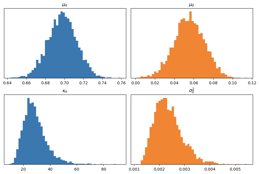
At first glance, we can see that, on average, the probability of making a first free throw is around 70%, and that second attempts are, on average, about 6% more likely to go in. While this isn’t a surprising result, it’s reassuring to see that the inferences from the hierarchical model are consistent with our previous findings.
What’s truly interesting about this hierarchical approach is that it allows us to analyze the posterior distributions of \(\pi_i\), \(\theta_i\), and \(\delta_i\) at the individual level — that is, for each player.
However, visualizing these distributions for all players can quickly become impractical. To make things more manageable, we selected a representative subset of players based on their \(N_1\) values (the number of first attempts). Specifically, we kept the 10 players with the highest \(N_1\), and from the remaining group, we sorted them from lowest to highest and chose every second player to form a more manageable sample.
| player_id | player_name | y_1 | y_2 | n_1 | n_2 |
|---|---|---|---|---|---|
| i32 | str | u32 | u32 | u32 | u32 |
| 1642264 | "Castle, Stephon" | 128 | 121 | 192 | 152 |
| 1642274 | "Missi, Yves" | 63 | 64 | 112 | 92 |
| 1642259 | "Sarr, Alex" | 62 | 50 | 88 | 77 |
| 1642268 | "Collier, Isaiah" | 56 | 49 | 85 | 69 |
| 1642258 | "Risacher, Zaccharie" | 55 | 47 | 82 | 62 |
| 1642271 | "Filipowski, Kyle" | 47 | 46 | 81 | 62 |
| 1641744 | "Edey, Zach" | 54 | 36 | 76 | 51 |
| 1642377 | "Wells, Jaylen" | 62 | 44 | 73 | 56 |
| 1641842 | "Holland II, Ronald" | 51 | 41 | 70 | 52 |
| 1642270 | "Clingan, Donovan" | 33 | 29 | 60 | 44 |
| 1641824 | "Buzelis, Matas" | 45 | 43 | 59 | 49 |
| 1642273 | "George, Kyshawn" | 39 | 31 | 51 | 42 |
| 1642266 | "Walter, Ja'Kobe" | 34 | 32 | 47 | 36 |
| 1642347 | "Shead, Jamal" | 32 | 20 | 42 | 26 |
| 1641783 | "da Silva, Tristan" | 29 | 26 | 35 | 28 |
| 1642272 | "McCain, Jared" | 23 | 23 | 28 | 25 |
| 1642348 | "Edwards, Justin" | 17 | 15 | 24 | 22 |
| 1641810 | "Reeves, Antonio" | 16 | 12 | 21 | 14 |
| 1631232 | "Brooks Jr., Keion" | 12 | 10 | 17 | 13 |
| 1642277 | "Furphy, Johnny" | 11 | 7 | 13 | 9 |
| 1641736 | "Beekman, Reece" | 8 | 8 | 11 | 10 |
| 1642265 | "Dillingham, Rob" | 4 | 4 | 9 | 6 |
| 1630574 | "Hukporti, Ariel" | 2 | 4 | 7 | 6 |
| 1630283 | "Kelley, Kylor" | 1 | 5 | 5 | 5 |
| 1641989 | "Harkless, Elijah" | 2 | 1 | 3 | 3 |
| 1630762 | "Wheeler, Phillip" | 1 | 1 | 1 | 1 |
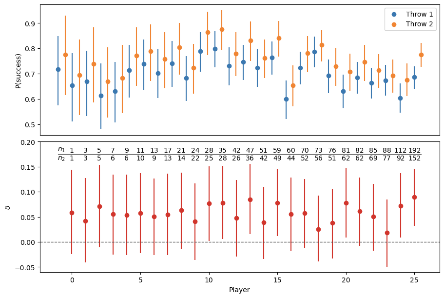
We can then visualize the marginal posteriors of \(\pi_i\), \(\theta_i\), and \(\delta_i\) for each selected player. Naturally, as the number of observed shots increases, the posterior distributions become narrower, reflecting a higher level of certainty.
In every case, even when \(N_1 = 1\) and \(N_2 = 1\), the posterior mean of \(\theta_i\) is greater than that of \(\pi_i\).
From another perspective, the bottom panel shows that the mean of \(\delta_i\) is always greater than 0. However, it’s only in cases where we have hundreds of attempts that we can conclude, with probability close to 1, that players are indeed better on their second attempts than on their first.
Since we’re Bayesians and use Markov Chain Monte Carlo methods to obtain samples from the posterior, we can compute, for each player, the probability that \(\delta_i\) is greater than 0. With these probabilities, we can build the following summary histogram:
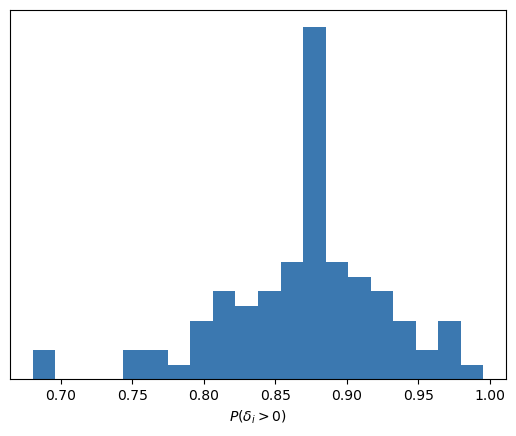
Then, no matter which rookie we look at, we’ll always conclude that they have a moderate to high probability of being more effective on their second free throws than on their first.
Finally, let’s compare the posterior distribution of \(\delta\) from the pooled model with the posterior of \(\mu_\delta\) from the partially pooled model, since both represent the same quantity: the average difference in success probability between a second and a first attempt.
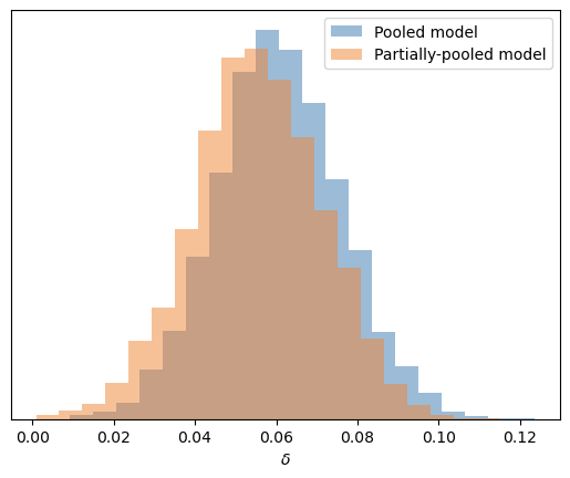
Fortunately, there are no surprises to report. Both models lead us to practically the same conclusions about the average \(\delta\), although it’s worth noting that in the hierarchical model, the posterior is slightly more regularized toward 0 compared to the pooled model.
However, we shouldn’t forget that using a hierarchical model allowed us to obtain posterior distributions for each individual player.
Examples like this are what remind me why I enjoy the Bayesian approach to statistical modeling so much.
While we could have settled for a simple hypothesis test, like the one presented in the article mentioned above, the flexibility offered by tools like PyMC allows us to go several steps further.
We proposed a hierarchical model (not a trivial one), implemented it in PyMC, and then, together with nutpie, used it to obtain samples from the posterior.
From those samples, we were able to draw several interesting conclusions. Not only the global ones, which confirm that basketball players tend to miss their first free throws more often than their second (consistent with the article’s findings), but also player-specific insights.
And above all, beyond the practical usefulness of the model or the insights we can extract… isn’t it just incredibly fun to play Bayes?